其实是初中数学的内容。

研究高斯软件的并行效率时,作者根据公式

$ s = n \times (1.015 - n \times 0.0067) $

得出了「并行核数大概在75的时候达到最大速度」。我突然有点糊涂了,这个结论是怎么得出的呢?

明显这是一个初中数学问题,因为函数是个一元二次函数,有公式,可惜我已经忘光光了。用数形结合的思路

1
2
3
4
5
6
7
f = @(x) -0.0067 * x.^2 + 1.015 * x;
x = 1:100;
plot(x, f(x));
xl = xlabel("n", "Units", "Normalized", "Position", [0.5 -0.07786 0]);
yl = ylabel("s", "Units", "Normalized", "Position", [-0.1 0.5 0]);
set(xl, "FontSize", 30); set(yl, "FontSize", 36);
print("n(1.015-n0.0067).ps", "-color");

s = n × (1.015 - n × 0.0067)

可以看出大概是75的时候效率最大,这时我也大概想起了公式是啥样的。不行,这个问题要一般话,要用专门的工具解决:

1
2
phi = @(x) 0.0067 * x^2 - 1.01 * x;
sqp([1], phi)

这里用Octave的sqp()函数求了phi()的最小值,这个phi()就是上面公式的值乘以−1,也就是把求最大值转换为求最小值,其他的量都默认,从1开始找最小值,求得的结果是75.373。

又是一次脱裤子放屁的经历。收获是又玩了一把Octave,但这个方法的价值不局限在这里,因为如果函数更为复杂,没有公式,图形又不好看,还需要精确求解的时候,该方法的优势就体现出来了。

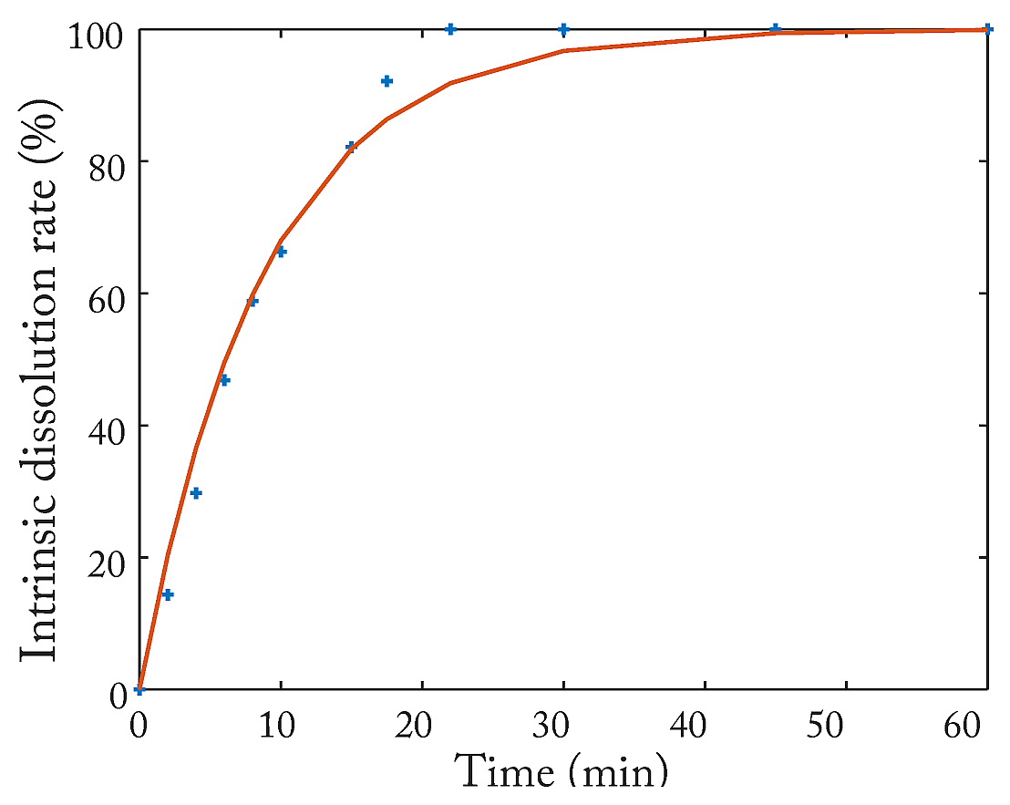
举个栗子,某种药物的释放程度随时间变化,t分钟时释放比例以P表示,得到的数据是

1
2
t = [0 2 4 6 8 10 15 17.5 22 30 45 60];
P = [0 0.1435 0.29768 0.46835 0.58834 0.66296 0.82152 0.9215 1 1 1 1 ];

如果以如下的模型来拟合这些数据

$ P = 1 - e^{-K \times t} $

看不出来了吧,我可以拟合

1
phi = @(K) abs(sum(P) - sum(1 - exp(-K * t))); sqp([0.01], phi)

结果是0.11390,画图

1
2
3
4
5
6
7
8
plot(t, P * 100, '@');
K = 0.11390;
hold on;
plot(t, (1 - exp(-K * t)) * 100);
xl = xlabel("Time (min)", "Units", "Normalized", "Position", [0.5 -0.07786 0]);
yl = ylabel("Intrinsic dissolution rate (%)", "Units", "Normalized", "Position", [-0.1 0.5 0]);
set(xl, "FontSize", 24); set(yl, "FontSize", 26);
print("Fit.ps", "-color");

Fit

这两个图都用了一些技巧,除了坐标的位置动过外,还改了PostScript文件,怎么改另写一篇文章介绍咯。

2019-01-18 Update:

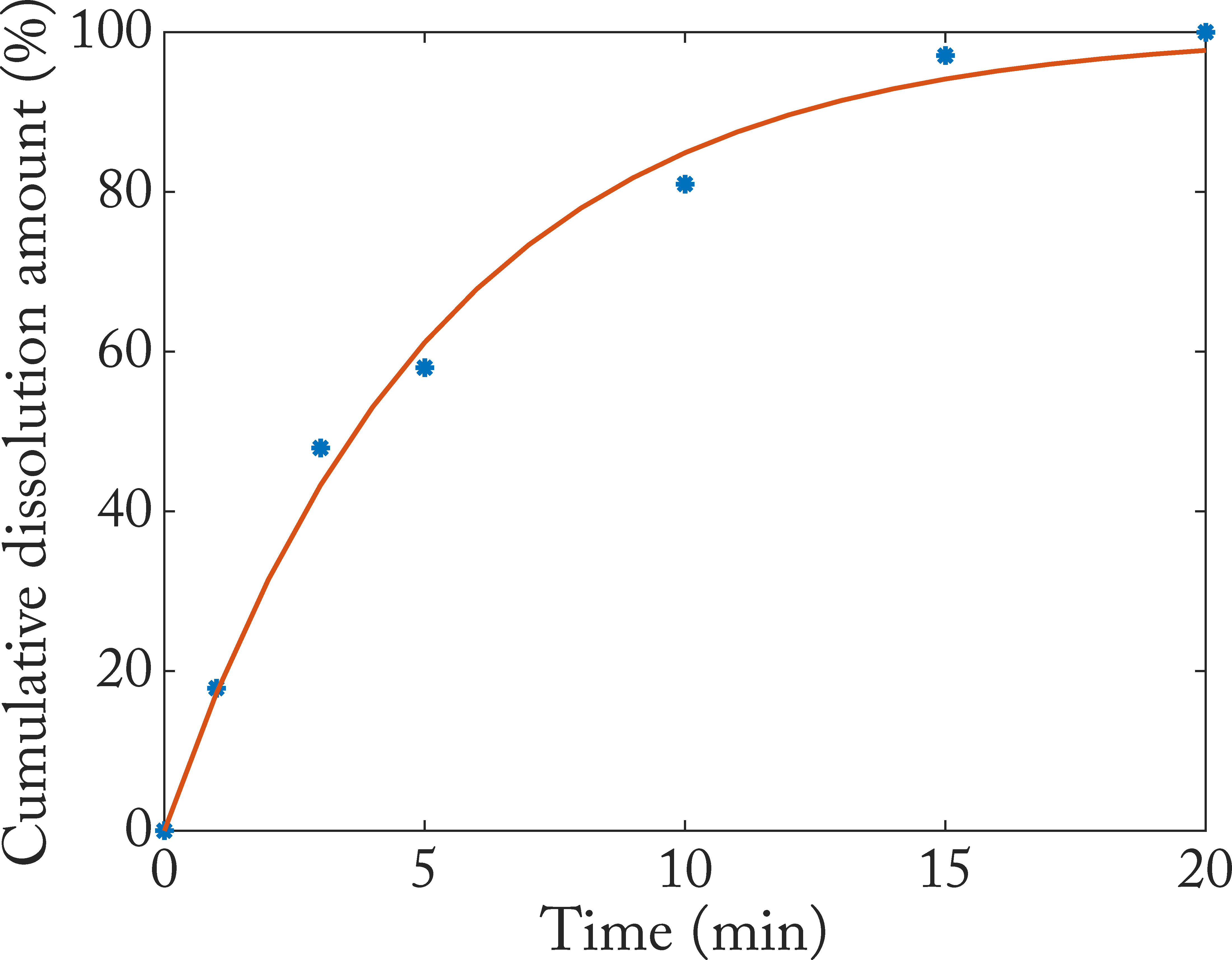
除了上面说的方法外,还可以用optim包里的函数进行优化:

1
2
3
4
5
6
7
8
9
10
11
12
t = [0 1 3 5 10 15 20];
P = [0.00000 0.17856 0.47929 0.57990 0.80975 0.97066 1.00000];
ffun = @(x, p) 1 - exp (-p (1) * x)
pkg load optim
[f, p, cvg, iter, corp, covp, covr, stdresid, Z, r2] = leasqr(t, P, [0], ffun)
plot(t, P, '*');
hold on;
plot([0:20], ffun([0:20], p));
xlabel("Time (min)");
ylabel("Cumulative dissolution amount (%)");
set(gca, 'yticklabel', [get(gca, 'ytick') * 100]);
print("a.svg");

Fit

2019-07-05 Update:

补一个做logistic拟合的代码。

1
2
3
4
5
6
7
8
9
10
11
12
13
14
15
16
17
18
19
20
21
22
23
24
25
26
27
28
29
30
31
32
33
34
35
data = [
0.0 12 0
50 12 0
100 12 0
300 6 6
400 4 8
500 12 0
1000 12 0
];

dose = data(:, 1);
death = data(:, 3) ./ (data(:, 2) + data(:, 3));

ffun = @(x, P) (P(2) + ((P(1) - P(2))./(1 + (x / P(3)).^P(4)))) # y = A2 + (A1-A2)/(1 + (x/x0)^p)
pkg load optim;

[f, p, cvg, iter, corp, covp, covr, stdresid, Z, r2] = leasqr(dose, death, [0.2 0.2 0.2 0.2], ffun)
fun = @(x) (ffun(x, p) - 0.5);
x50 = fzero(fun, 300)
x50 *= ones(1, 2);
y50 = [-0.5 1.5];

plot(dose, death, 'bo');
hold on;
plot(x50, y50, 'b--')
plot_range = linspace(min(dose) * 0.8, max(dose) * 1.2, 20);
plot(plot_range, ffun(plot_range, p), 'r-')
ybounds = [0 1.09];
ylim(ybounds);
set(gca(), 'ytick', ybounds(1):0.2:ybounds(2));
new_yticks = [cellstr(num2str(get(gca, 'ytick')' * 100))];
set(gca(), 'yticklabel', new_yticks);
# xlim([-1 700]);
xlabel('Dose (mg/Kg)');
ylabel('Mortality rate (%)')